In my last post, I attempted to derive an online update formula for the attention mechanism. However, the resulting formula isn’t optimal for high-performance real-world implementations. There are two issues left undiscussed:
- Granularity of the Computation: The formula treats the query as a vector, which is too granular. In practice, it’s better to work with matrices, as this allows leveraging specialized hardware like tensor cores in GPUs to speed up matrix multiplication.
- Numerical Stability: There are smarter ways to reduce computational load and enhance numerical stability.
Let’s address these issues in this post.
Table of Contents
Recap the Three-Stage Online Updated Attention
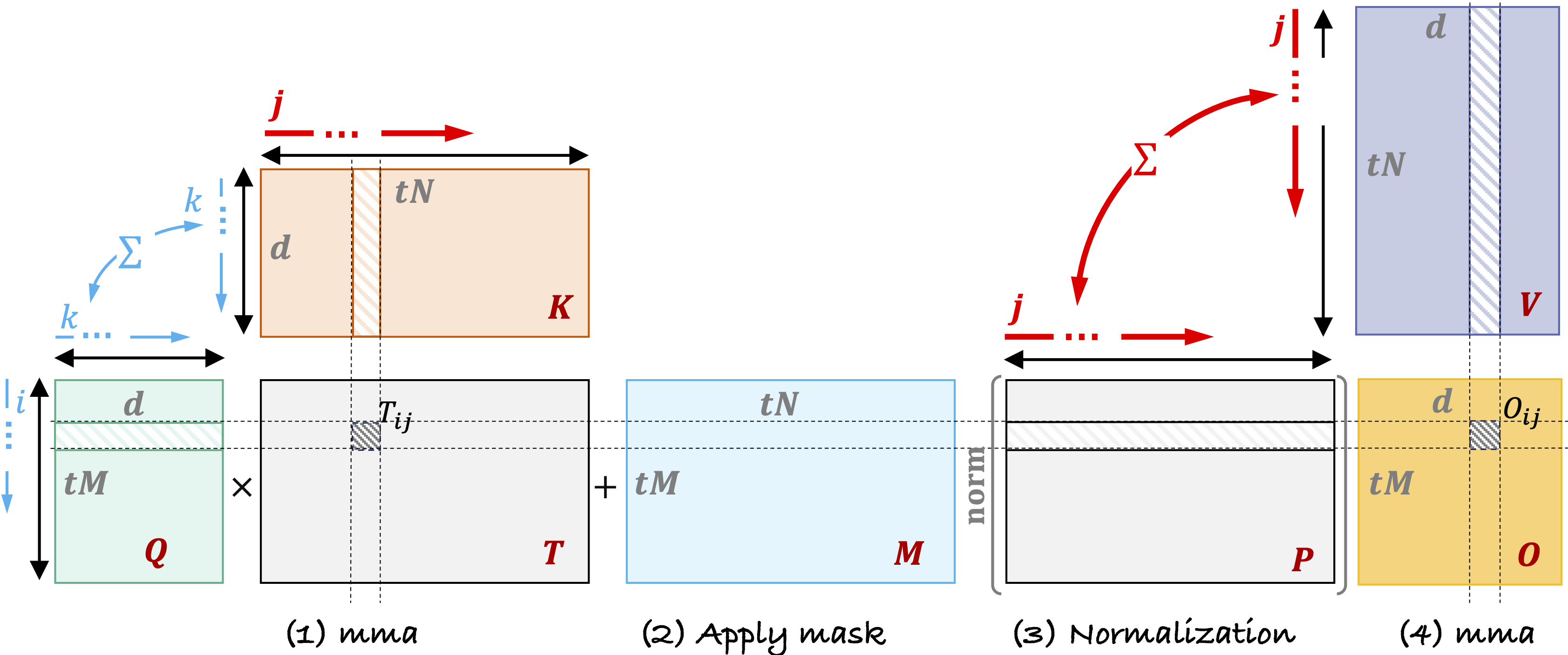
Let’s recap the attention formula for calculating $\vec{o_i}$. Figure 1 shows a chunk of the query, key, mask, and value matrices, along with the notation used.

Fig.1 Query-Key-Mask-Value Matrix Visualization and Notation
In Fig 1, the $j$-annotated dimension highlighted in red represents sequence length and carries data dependencies over the entire sequence. Below we give the formula for the attention mechanism corresponding to Fig 1.
\[\begin{align*} T[i,j] &= \sum_k \left(Q[i, k] * K [k,j]\right) & [tM, tN] &= \sum_k \left([tM, d]\ *\ [d, tN] \tag{1}\right)\\ ---&-----------&---------&-----------\\ S &=T + M & [tM, tN] &= [tM, tN] + [tM, tN] \tag{2}\\ ---&-----------&---------&-----------\\ \color{#1E90FF}{\vec{C}_i} &= \max_{\color{#FF0000}{j}} \left(S[i,\color{#FF0000}{j}] \right) & [tM,1]&=[tM, tN] \tag{3}\\ \bar{S} &= \exp \left( S - \vec{C}_i \right)&[tM, tN] &= [tM, tN] - [tM,1]\\ \color{#1E90FF}{\vec{L}_i} &= \sum_{\color{#FF0000}{j}} \bar{S}[i, \color{#FF0000}{j}] &[tM, 1] &= [tM, tN]\\ \vec{P}_i &= \frac{\bar{S}}{\color{#1E90FF}{\vec{L_i}}} & [tM, tN] &=\frac{[tM, tN]}{[tM, 1]}\\ ---&-----------&---------&-----------\\ \color{#1E90FF}{O}[i,d] &= \sum_{\color{#FF0000}{j}} \left( P[i,\color{#FF0000}{j}]\ * \ V[\color{#FF0000}{j},d] \right )& [tM, d] &= [tM, tN]\ @ \ [tN, d] \tag{4} \end{align*}\]Flash attention refactors this computation into three stages, motivated by the fact that the sequence-wise normalized softmax operation has an online updated equivalent. This allows computation to occur in a three-stage streaming manner by maintaining running statistics. The three stages are:
-
Local Compute Stage: The attention function is computed locally within each chunk, independent of others, with rescaling based on running statistics.
-
Statistics Update Stage: Running statistics are updated for numerical stability across the sequence.
-
Global Rescaling Stage: After all chunks are processed, the final output is rescaled based on the accumulated running statistics.
This streaming approach enables efficient computation of attention without the need to store large intermediate matrices back in slow external memory. The online update formula for the running statistics must be derived based on the original attention formula for three values:
- The running maximum values $\color{#1E90FF}{\vec{C}_i}$.
- The running normalization denominator values in the softmax operation $\color{#1E90FF}{\vec{L}_i}$.
- Based on $\color{#1E90FF}{\vec{C}_i}$ and $\color{#1E90FF}{\vec{L}_i}$, the formula for the output $\color{#1E90FF}{O}$ also needs to be derived.
Here’s how we derived them in the last post:
\[\begin{align*} &\vec{C}_i^{\ t} = \max \left( \vec{C}_i,\ \color{#1E90FF}{\vec{C}_i^{\ t-1}} \right) \\ ---&-------------------\\ &\Delta \vec{C}_i^{\ t} \triangleq \vec{C}_i - \vec{C}_i^{\ t} \\ &\Delta \vec{C}_i^{\ t-1} \triangleq \color{#1E90FF}{\vec{C}_i^{\ t-1}} - \vec{C}_i^{\ t} \\ &\vec{L}_i^{\ t} = \vec{L}_i \exp \left(\Delta \vec{C}_i^{\ t} \right) + \color{#1E90FF}{\vec{L}_i^{\ t-1}} \exp \left(\Delta \vec{C}_i^{\ t-1} \right) \\ ---&-------------------\\ &O^{t} = \frac{\vec{L}_i \exp \left(\Delta \vec{C}_i^{\ t} \right)O + \color{#1E90FF}{\vec{L}_i^{\ t-1}} \exp \left(\Delta \vec{C}_i^{\ t-1} \right) \color{#1E90FF}{O^{t-1}}}{\vec{L}_i^{\ t}} \end{align*}\]The Log-Sum-Exp Trick and Numerical Stability
Before we proceed, let’s take a moment to discuss the log-sum-exp (LSE) trick. The softmax function normalizes an $N$-dimensional vector $x$ into a probability distribution $\vec{p}=\left[p_1, p_2, \cdots, p_N\right]$ as follows:
\[p_i = \frac{\exp \left(x_i\right)}{\sum_{j=1}^N \exp \left(x_j\right)}, \quad \sum_{i=1}^N p_i = 1 \tag{eq.1}\]Dealing with exponential operations can be prone to numerical underflow or overflow. To address this, let’s consider computing the log probability $\log p_i$ instead:
\[\begin{align*} \log p_i &= \log \left(\frac{\exp \left(x_i\right)}{\sum_{j=1}^N \exp \left(x_j\right)}\right) \\ &=x_i - \log \left(\sum_{j=1}^N \exp \left(x_j\right)\right) \end{align*}\]Then we have $p_i$ as:
\[\begin{align*} p_i &= \exp \left(x_i - \underbrace{\log \left(\sum_{j=1}^N \exp \left(x_j\right)\right)}_{LSE} \right) \tag{eq.2} \end{align*}\]From $\text{eq}.1$ and $\text{eq}.2$ we can see that the LSE operation can be used to normalize the values in the denominator of the softmax function. However, you might wonder if this is really helpful for numerical stability since we are still computing the exponential operation.
To address this concern, let’s consider normalizing the input values for LSE first. By doing so, we effectively reduce the range of the exponentials before performing the exponential operation. This helps prevent the exponential terms from becoming too large (leading to overflow) or too small (leading to underflow), thereby ensuring numerical stability.
\[\begin{align*} L &= \log \left(\sum_{j=1}^N \exp \left(x_j\right)\right) \\ e^{L} &= \sum_{j=1}^N \exp \left(x_j\right) \\ e^{L} &= e^c\sum_{j=1}^N \exp \left(x_j - c\right) \\ L &= c + \log \left(\sum_{j=1}^N \exp \left(x_j - c\right)\right) \end{align*}\]From the above formula, we can see that the LSE operation is advantageous because we can shift the values of $x_j$ by a constant $c$ while still computing the same final result. If we set $c$ to the maximum value of $x_j$, we ensure that the largest positive exponential value is $\exp(0)=1$, and the largest negative exponential value is $\exp(-\infty) = 0$. This helps prevent overflow and underflow in the exponential operation, thus enhancing the numerical stability of the softmax operation’s normalization factor.